Video Vision Transformer (ViViT)
We select ViViT-B/16×2 FE (A ViT-Base backbone with a tubelet size of \(h\times w\times t = 16\times16\times2\), FE represents factorised encoder) as the backbone of our model.
In the original paper, there are four sort of Multi-Head Self-Attention (MHSA) modules (TE, FE, TFE, and FTE).This work selected FE because ViViT-B/16×2 FE performed the best of all four versions of ViViT-B/16×2.
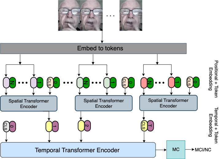
The figure shows that in ViViT, the Transformer Encoder takes the combined positional and embedded cubic tokens as input, and it contains Self-Attention module followed by the FeedForward module. This formula presents the details of the input tokens.
\(\mathbf{z}=[z_{cls},\mathbf{E}x_{1},\mathbf{E}x_{2},\dotsm,\mathbf{E}x_{n_{h}n_{w}n_{t}}]+\mathbf{p}\),
where \(z_{cls}\) is a learnable class token, \([x_{1},x_{2},\dotsm,x_{n_{t}n_{h}n_{w}}]\) is the tensor of the cubic patches, \(x_{i}\in \mathbb{R}^{h\times w\times t}\) \(n_{h}n_{w}n_{t}\) is the number of cubic patches. \(E\) is the linear projection to embed cubic patches. In addition, \(\mathbf{p}\in \mathbb{R}^{n_{h}n_{w}n_{t}\times d}\) represents a learnable positional embedding. \(d\) is the dimension of the embedded token.
Given the layer l, the Self-Attention module consists of Layer Normalization (LN) and Multi-Head Dot-Product Attention, while the FeedForward (FF) module includes LN and MLP. Both modules use skip-connection to enrich features and prevent gradient vanish. The follow Equation shows that FE has two parts, Spatial Transformer Encoder (\(L_{s}\)) and Temporal Transformer Encoder (\(L_{t}\)).
- Spatial Transformer Encoder extracts the latent representations on the different tokens with the same temporal index, called spatial features.
- Temporal Transformer Encoder studies the interactions between latent representations from different time steps, called temporal features.
Assuming that the \(L_{s}\) and \(L_{t}\) repeats \(n_{sp}\) and \(n_{tp}\) times. FF processes the output of FE and returns Sequence-Level Spatio-Temporal feature. The above explanation can be summarized as the follows.
\[\begin{align} \mathbf{y}^{l}_{s} &= L^{l}_{s_{n_{sp}}}(\dotsm L^{l}_{s_{1}}(LN(\mathbf{z}^{l}))\dotsm) \label{eq:fe.1}\\ \mathbf{y}^{l}_{t} &= L^{l}_{t_{n_{tp}}}(\dotsm L^{l}_{t_{1}}(\mathbf{y}^{l}_{s})\dotsm) \label{eq:fe.2}\\ \mathbf{y}^{l}_{FE} &= \mathbf{y}^{l}_{t} + \mathbf{z}^{l} \label{eq:fe.3}\\ \mathbf{y}^{l}_{FF} &= MLP(LN(\mathbf{y}^{l}_{FE})) + \mathbf{y}^{l}_{FE} \label{eq:fe.4} \end{align}\]